A Guide to Creating Dynamic Links for Tasks in Google Sheets

---

After creating the Todo lists in our guide to creating todo lists, we realized that our team members still have to go back to the Tasks tab to update the task's status. As that Tasks tab gets larger, it'll become more difficult to search for that specific task. In this guide, we'll set up some hyperlinks to make it easier to find the task they need to update.

Setting up the Link

The Base URL

Every Google Sheet URL has a unique ID associated to it. Let's take our "Task Management - Template" file for example:

https://docs.google.com/spreadsheets/d/13nPGTSNKwv_VCJR3DDalsyuEpFjlnQCShWZyZqZ5hQQ/edit

The ID here is 13nPGTSNKwv_VCJR3DDalsyuEpFjlnQCShWZyZqZ5hQQ.

When you copy down the URL to share with colleagues, you'll sometimes see a gid= attached to the URL. This is the ID for the tab. In addition to allowing you to link people directly to a specific tab on a Google Sheet, you can also send them directly to a specific Cell. You can do this by using the range= parameter, which accepts A1 Notation - e.g. C2.

Your Link should end up looking something like this:

https://docs.google.com/spreadsheets/d/13nPGTSNKwv_VCJR3DDalsyuEpFjlnQCShWZyZqZ5hQQ/edit#gid=1746393838&range=C2

Using the "ADDRESS" Formula

Now that we have the URL structure figured out, how can we use it across the entire Tasks tab? If you were thinking about doing something like this:

="https://docs.google.com/spreadsheets/d/13nPGTSNKwv_VCJR3DDalsyuEpFjlnQCShWZyZqZ5hQQ/edit#gid=1746393838&range="&C2

and copying it down all of the rows, you're not going to have a good time.

Since the range requires an A1 Notation, using C2, C3, C4, etc won't work in the URL since it'll just return the value of those cells. What we need to use here is the =ADDRESS() formula.

The =ADDRESS() formula can be set up to give you the A1 Notation of a specific cell. It takes in 5 paramters into it:

• Row
• Column
• Absolute Mode
• Use A1 Notation?
• Sheet

The first 2 are required and the others are optional. We're going to use the first 4 in this guide.

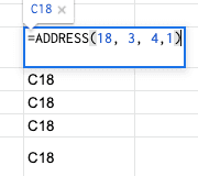
The Row and the Column parameters need to be numbers, so we'll have to get the index of of them using the =ROW() and =COLUMN() formulas. Before we do that, try typing this formula into a cell to see what it gives you: =ADDRESS(18, 3)

You'll probably see $C$18 as the output of that formula. For our purposes, we don't want it to have those $ signs which basically just means that it's an absolute value. For the Absolute Mode parameter, it accepts these options:

• 1: Row absolute & Column absolute
• 2: Row absolute & Column relative
• 3: Row relative & Column absolute
• 4: Row relative & Column relative

We'll go with 4 in our formula so that both the row and column are set to relative.

Your formula should look like this now: =ADDRESS(18, 3, 4) and it should output C18. If you hover over it, you'll see that it gives you a sneak peak to what's in cell C18 (this doesn't happen when the row & column are absolute).

The last parameter is the A1 Notation, which we'll just want to set to TRUE (or 1 to make it simple). The new formula should read: =ADDRESS(18, 3, 4, 1).

When you copy down this address formula, you'll notice that it doesn't dynamically change - meaning the output won't read C18, C19, C20, etc. In order to do this, we'll need to use the =ROW() and =COLUMN() formulas from earlier.

Using References Cells

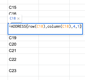
What we'll do here is replace the Row and Column parameters with the =ROW() and =COLUMN() formulas. So instead of 18, you'll have ROW(C18) and instead of 3 you'll have COLUMN(C18). Your formula will look like this when you're done:

=ADDRESS(row(C18),column(C18),4,1)

If you copy this formula down multiple rows, you'll see that it will dynamically change its output to match with the row now.

Creating the Full URL

Now that you have a dynamic list of referenced cells, it's time to combine it with the base URL from earlier. This part is fairly simple. You can do with this the =CONCAT() formula, or the =CONCATENATE() formula, or just with an Ampersand & between the values. Here's how it'll look with an Ampersand:

="https://docs.google.com/spreadsheets/d/13nPGTSNKwv_VCJR3DDalsyuEpFjlnQCShWZyZqZ5hQQ/edit#gid=1746393838&range="&ADDRESS(row(C4),column(C4),4,1)

Congrats, you have what you need to link users back to the exact row on the Tasks tab. Take this formula and paste it into each row. Just use the next available column - if you've been following along this guide series, it'll be Column I.

Since we used the =QUERY formula for our Todo lists, these new hyperlinks will automatically show up! If you go back to one of your Todo lists, you'll see it displayed in the last column.

---

Future-proof the Column

Since you copied down the forumla, it'll only show up for things that already existed. Meaning, if you get a new task submission from the Google Form, it won't have the hyperlink attached to it. Not to worry though, there's a way to auto populate it regardless of how many new rows get inserted. The answer is the =ARRAYFORMULA() formula.

In short, this formula will take a large set of data and plug in a value down the entire row or column depending on what you have in it. For this scenario, it'll populate values down the entire column so that each row has the formula's output.

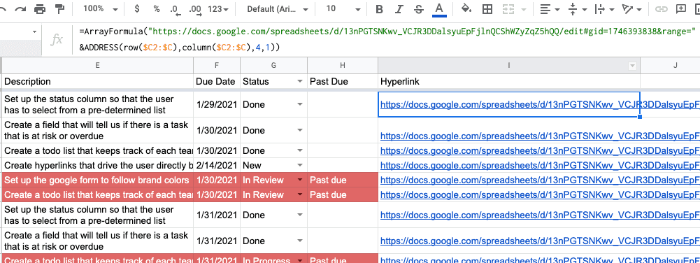
The first thing to do is to change our =ROW() and=COLUMN() formulas to look at ranges instead of a single cell. Change the C2 to C2:C. After that, wrap the entire thing in the ARRAYFORMULA() formula. It'll look like this:

=ArrayFormula("https://docs.google.com/spreadsheets/d/13nPGTSNKwv_VCJR3DDalsyuEpFjlnQCShWZyZqZ5hQQ/edit#gid=1746393838&range=" &ADDRESS(row(C2:C),column(C2:C),4,1))

If you get a #REF! error, that just means that you have to delete everything below the formula. The only things you should have populated into Column I is I1 for the column header, and I2 which should be the formula from above.

Thats it for this part of the Guide to building a Task Management tool in Google Sheets. In the next guide, we'll look into making it possible to make a task as done through the Todo list instead of the Tasks tab. Click here to continue onto the next part.