A Guide to Creating a Dynamic Alerts Column

---

When working with large sets of data, it can be hard to pinpoint the rows you're looking for. It's especially difficult when you have more than one set of criteria. In this guide, we're going to go through a few different ways to make it easier to find rows based on two conditions and make it so it dynamically updates itself according to your data set.

The Conditions

The "Time" Condition

A common use case is "Time". People like to see which rows were after a certain date, before a certain data, or between two dates. For our task management tool, we'll focus on things that are Past Due. To calculate that, we'll be using the "Due Date" column and comparing it against the current date.

To get the current date, we're going to use the =NOW() formula. Since this is a formula, it'll always reflect today's data.

Then we're going to compare this against our "Due Date" column, like this: =$F3 < NOW(). This should return "TRUE" or "FALSE" depending on the due date. It should look something like this:

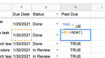
This is only half of the formula we need though. As you can see, it's showing "TRUE" for things that are already marked as done and that's not something we want to consider as "Past Due".

The "Status" Condition

Just like what we did for the "Time" condition, we'll use a basic formula to tell us if something is "Done" or not. The formula we'll be using is a simple "not equals" comparison. It'll look like this: =$G3<>"Done". Be sure to put your status in quotes.

Combining the Conditions

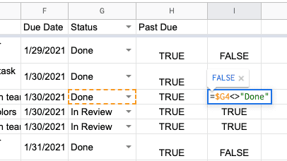
Now that we have both of the conditions working, it's time to combine them. There are many ways to combine the two, but we're going to use the AND() formula in this scenario. It'll look like this: =AND($F3<NOW(),$G3<>"Done")

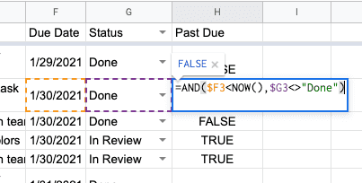
Congrats! Now you have a column dedicated to telling you if something is past its due date. We're not done though, scrolling through a list of TRUE and FALSE is still rough on the eyes. There's plenty that we can do to make it easier to scan through the list.

Transform the Text

An easy way to make it easier to scan through your list without straining your eyes over "TRUE" and "FALSE" is to just manipulate the text so that something different shows up. For example, only have it say "Past Due" if the comparison is "TRUE" and leaving it blank when it's "FALSE"

The IF statement

We're going to use the IF statement for this. It's fairly simple - the logic goes like this: If "this is true", then "do this", else "do this other thing". the formula itself is =IF(condition, output_if_true, output_if_false) and for our specific scenario, we'll replace "condition" with the formula we made above.

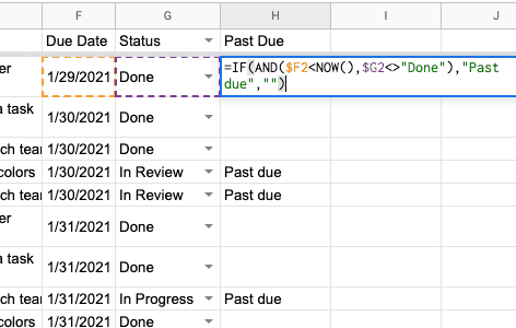
It should look like this when you're done: =IF(AND($F2<NOW(),$G2<>"Done"),"Past due","").

Notice how output_if_value is set to "" - meaning nothing, blank, nada. Having it blank helps with how you scan through the list. Here's what it'll look like:

Add Conditional Formatting

Sometimes just changing the text isn't enough though. For instance, what if you have multiple conditions that could result in "Past due", "At risk", or "Upcoming"? When you have multiple variations, adding in some colors will help. You can do this with conditional formatting, which is found under the "Format" option in the menu bar.

Highlight Matching Cells

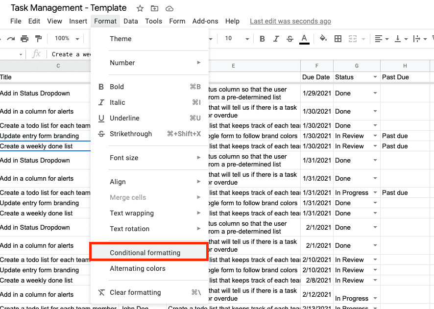
This is a pretty simple way to help you locate matching rows. It's also one of the faster ways of doing it which makes it a great "go-to" solution when you're short on time or just trying to quickly get it done.

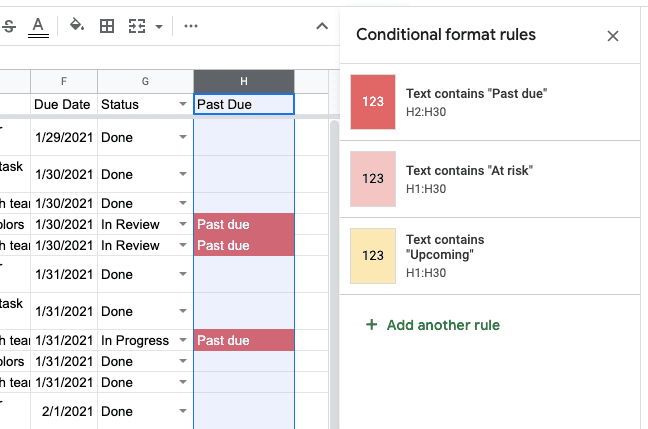
We'll set it up for the entire column and look for any text that matches up with "Past due". Make sure to put in the correct range in the "Apply to range" field. Then select "Text contains" from the dropdown menu for "Format rules". Put in "Past due" and then set up your "Formatting style" - we can just set it to the color red for now.

If you have multiple variations, just repeat this process and change out the text you're matching against. You can also set different colors and styles for each conditional rule. Once you're done, the conditional formatting tray will look like this:

Bypass the "Past Due" Column (OPTIONAL)

Want to get fancy and completely skip over the column? You can do that by using the formula in the conditional formatting rules. This will minimize the number of formulas you're using in the sheet and help keep things a bit cleaner for all you minimalists out there.

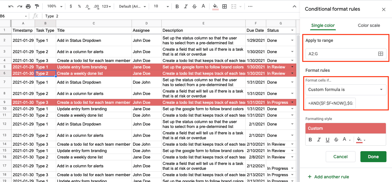
First thing you want to do is grab that =AND() formula we used earlier. We're going to use that as a custom formula in our conditional formatting rules. Once you have the formula, open up the conditional formatting tray and click on the "+ Add another rule" option. In the "Apply to range" field, you're going to use whatever range you want to highlight. If you want, you can also use multiple columns to give your entire row the formatting.

Under the "Format rules" dropdown, select the "Custom formula is" option. In the input field that appears, paste in the =AND() formula from before. Now change the $F3 and $G3 references to be absolute ranges for those columns. It'll should look like this: =AND($F:$F<NOW(),$G:$G<>"Done")

Set your formatting and you're done. You should see the entire row highlighted without the need for that separate "Past Due" column.

Creating a Report

Don't even want to bother with scanning through the list? You can create a filtered down report which will make it easier in general. There are two formulas that you can use for this. The =FILTER() formula and the =QUERY() formula.

The "Filter" Formula

The filter formula is a fast way to get a curated list of data based on 1 or many conditions. We can't use the same =AND() formula we made earlier, but it's still pretty simple. The format we need for this formula is (range, conditions...). Once you've put in the conditions, it'll look like this: =FILTER(Tasks, Tasks!$F:$F<NOW(), Tasks!$G:$G<>"Done")

Notice how it also filtered out the column headers? You could move the formula to call A2 and then paste in the headers to A1:H1, but there's better way than that - using the =QUERY() formula.

The "Query" Formula

The query formula is a very powerful formula if you know how to use it. We'll do a deep dive into it in another guide, but we'll go through the parts we need for this Past Due report.

The first step is setting up your query. The formula's format is: (range, select_query, headers). It'll look something like this: =QUERY(Tasks, "Select * Where A is not null", 1) - notice that "Tasks" doesn't have an A1 notation range, that's because we're using a Named Range here. Check out our guide on Named Ranges

This should give you a full list of the Tasks. Now we'll have to filter it down using some Where conditions. Let's tackle the "Status" condition first. The operator we'll want to use is the same as the what we used in the earlier formulas - <>. Your status condition will look like this: G <> "Done". -- note: case sensitivity matters here

When you add it into the query, it should look like this: Select * Where A is not null and G <> "Done".

The time condition is a little bit more complex, but here's the formula you'll need for it. We'll have a separate guide that talks about this formula in the future: F < date '" & TEXT(DATEVALUE(NOW()),"yyyy-mm-dd")& "'"

Once you put it all together, it should look like this: =QUERY(Tasks,"Select * Where A is not null and G <> 'Done' and F < date '" & TEXT(DATEVALUE(NOW()),"yyyy-mm-dd")& "'", 1) - where "Tasks" is a Named Range" and the "1" at the end means that there is 1 row designed as the header.

By using the =QUERY() formula, you can also apply sorting to it by adding Order by to the end of the select_query. For example, if you wanted to sort the results by the Assignee, you'd add in Order by D asc to the end. asc stands for Ascending order and desc for Descending order. For multiple sort criteria, just use a comma - like this: Order by D asc, F desc

That's it for this guide. If you made it this far, you should have a list of tasks that takes in new entries via a Google Form, dropdowns for selecting a status, conditional formatting to highlight any tasks that are Past Due, and also a separate report that you can use to monitor those past due tasks.

In the next part of this series, we'll set up custom todo lists for the assignees. Check out the guide here