A Guide to Basic Task Management with Google Sheets

---

Being able to manage your team's tasks is vital part to keeping the ship running. There are tons of tools out there, some free and others paid. Free is great until you realize you can't customize them to your specific needs or start to hit their limitations. The paid ones are usually good, but they're usually billed at a per-user amount so your monthly overhead starts to inflate quickly. Not exactly great for your runway.

In this guide, I'm going to show you how to use Google Sheets to create a task management tool that will serve you for a long time - at least until you're making enough money to justify one of the fancier solutions.

Why Google Sheets?

• It's free
• It supports simultaneous collaboration
• Built-in version control
• You can easily integrate it with other Google Products - such as Forms, Scripts, and Data Studio
• It supports up to 5,000,000 cells.
• Naturally comes with access controls and user permissions
• It's 100% customizable

Setup

• Create a new Google Sheet (you can do this through Google Drive, or just type in "sheets.new" into your browser's web address bar)
• Add in a new tab to the Google Sheet, you should have two tabs in total now. Rename them so that one is called "Settings" and the other is called "Dashboard"
  

Create an Entry Form

Google Forms

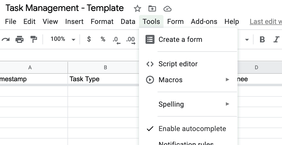
Since you're using a Google Sheet, you get the bonus of being able to directly link it to a Google Form. To set this up, go to the "Tools" option in the menu bar and select "Create a form". This will take you to a brand new Google Form which is automatically be connected with your Google Sheet.

Fill out your form with the questions you need to capture for each task. Typical things would be: "Title", "Description", "Assignee", "Due Date", and "Status". Google Forms has a bunch of different options for question types, so feel free to take your time playing with the form. Try out some single-select questions, paragraph questions, dropdowns, date fields, etc.

Connecting to Sheets

Once you're done with your form, head back over to your Google Sheet. You'll notice that you have 3 tabs in total now. The new one is called "Form Responses 1" and it's some that was auto-generated to capture and entries to the Google Form you just make. Go ahead and rename that to "Tasks" for now.

Enhance your Status column

Make the Column

If you added "Status" to your form, great. If you didn't, you'll have to add it as a new column - do that under your "Tasks" tab.

Add in a Dropdown

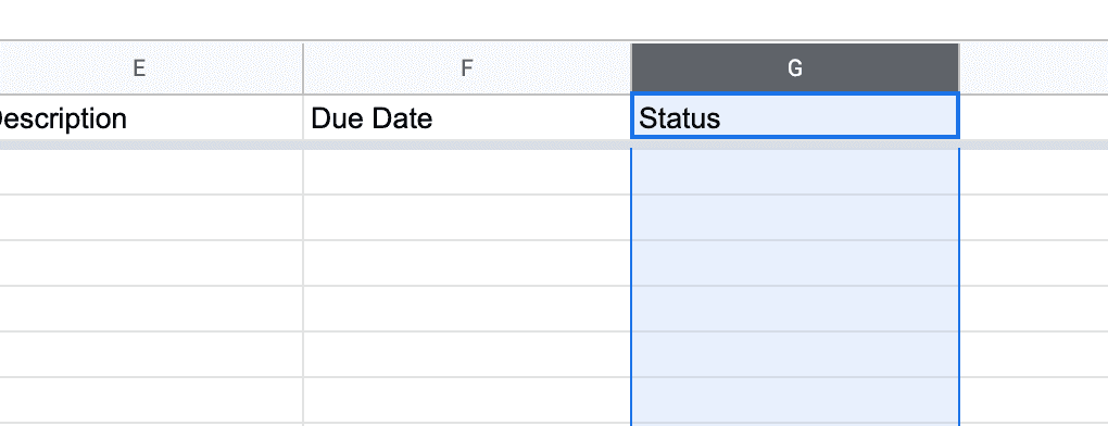
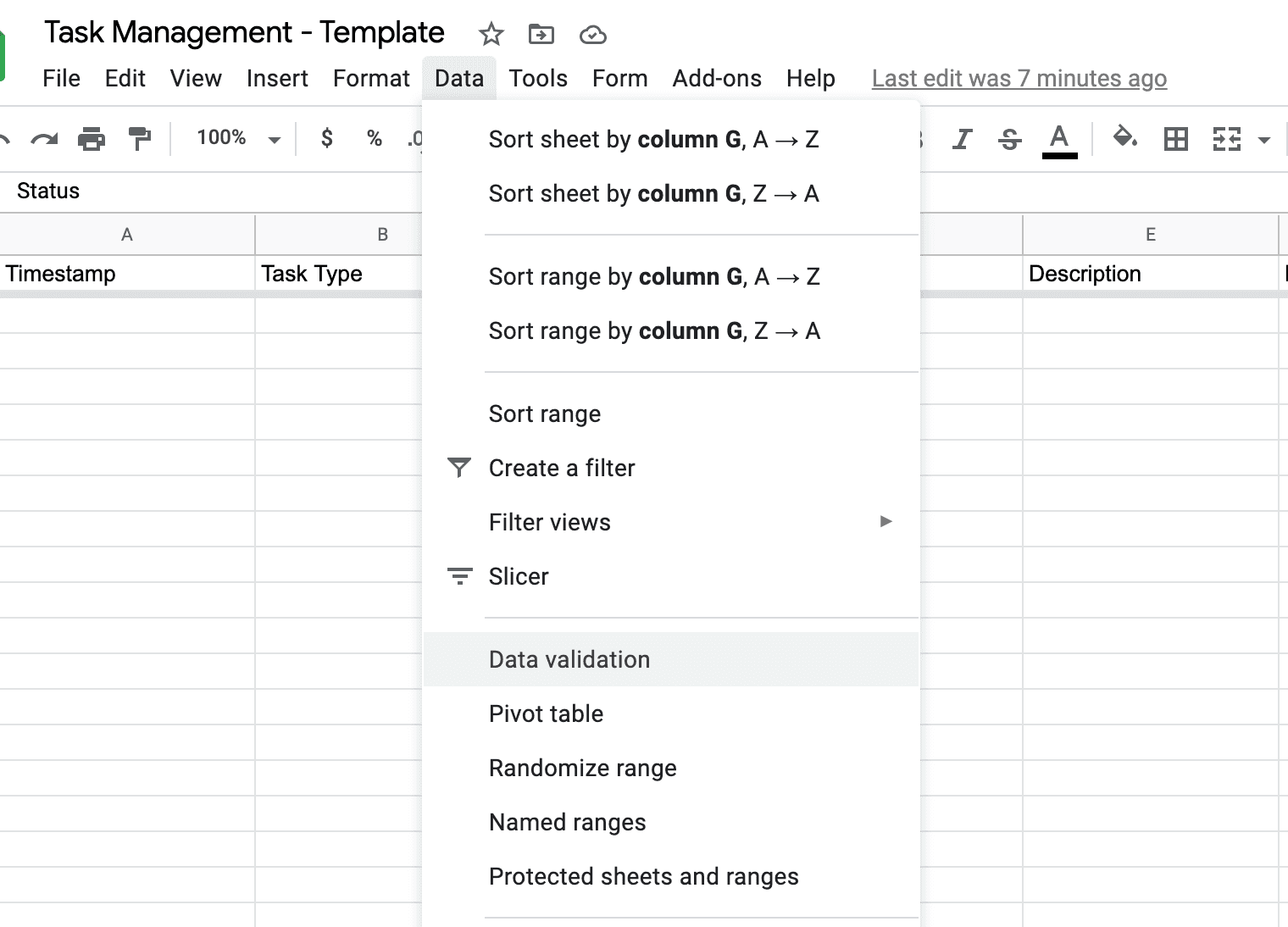
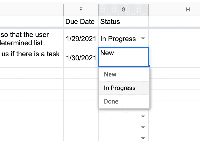
Once you have a "Status" column, it's time to fool-proof the field by making it into a dropdown. Click on the "Data" option in the menu bar and select "Data Validation"

For the "Cell range" field, put in the column range for your "Status" field. Make sure to start from row 2 so that you don't apply the dropdown to your column header. In your "Criteria" field, select "List form a range" as the option and then put in your status options into the input field - using commas to separate each option.

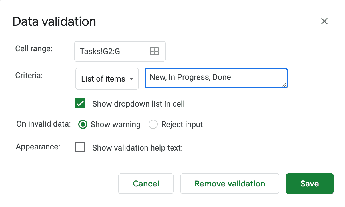
Congrats! You now have a dropdown for your status field that will help keep everything clean even if you have multiple people working in here.

Reporting

Now that you have a clean data set, you can report off of it cleanly. In this guide, we'll go through a basic way to report on tasks - count of tasks by assignee and status. The output is going to look like a matrix table

Add a Pivot Table

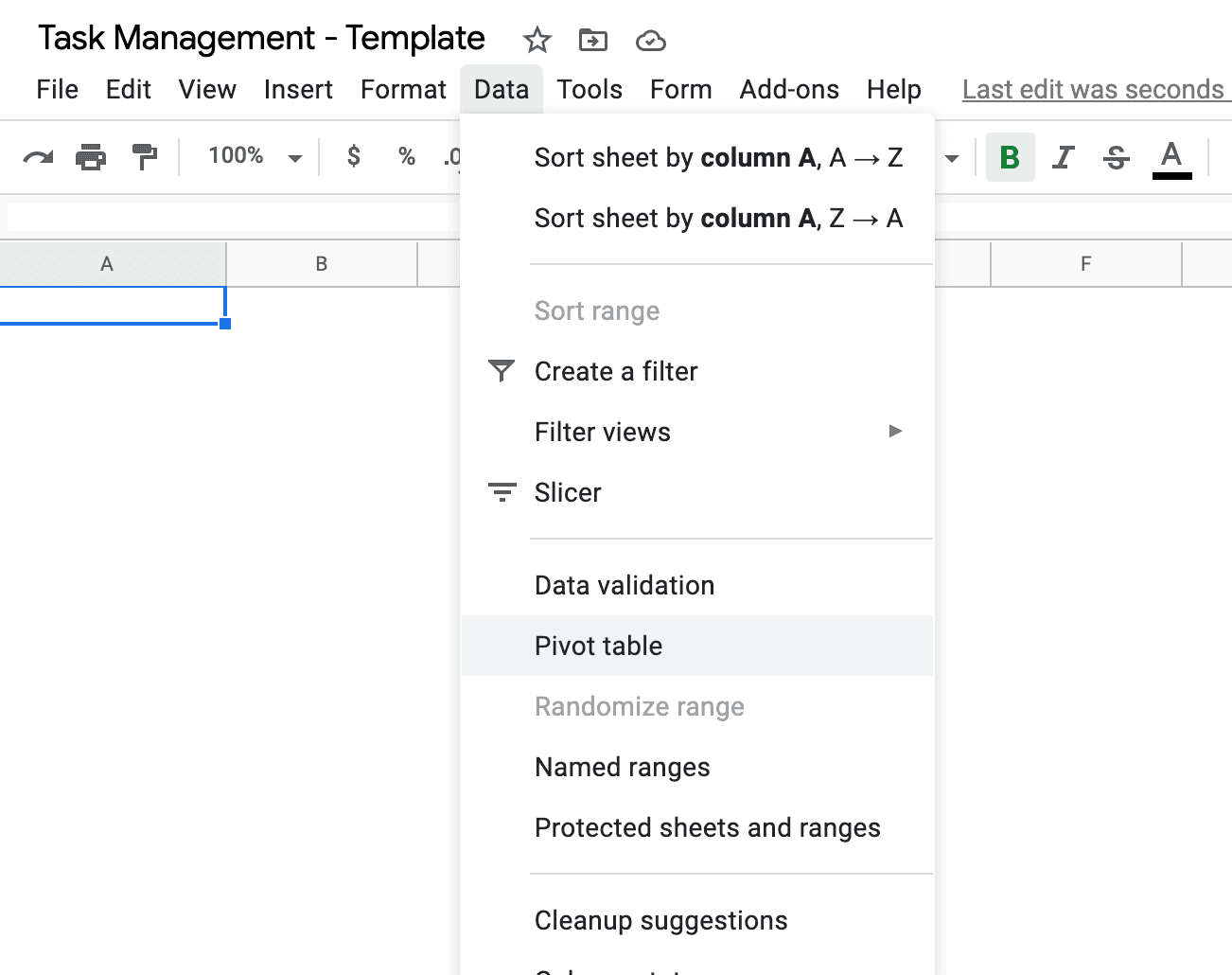
First, let's navigate back to the "Dashboard" tab. This is where you're going to put all of the aggregated metrics. Once you're here, go to the menu bar, select the "Data" option, and then select the "Pivot table" option.

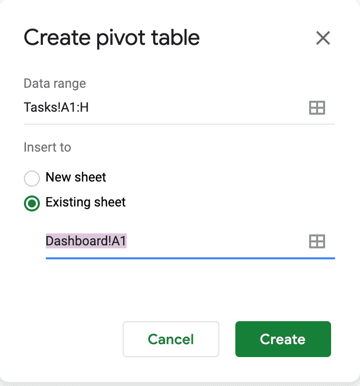
In the "Create pivot table" form, in the "Data Range" field, put in the location of your tasks - it should be something like "Tasks!A:H".

Adjust the settings

Then select to insert it into the "Existing sheet" and put in "Dashboard!A1" as the input. Once you hit the create button, it'll generate a pivot table that reads off of your tasks list. On the right hand side, you'll see a bunch of options. Select "Assignee" as your Rows, "Status" as your Columns, and "Status" as your Values.

Clean it up

You'll probably see that there is a blank column for your statuses. to remove that, select the "Filter" option and deselect "(Blanks)" from the dropdown.

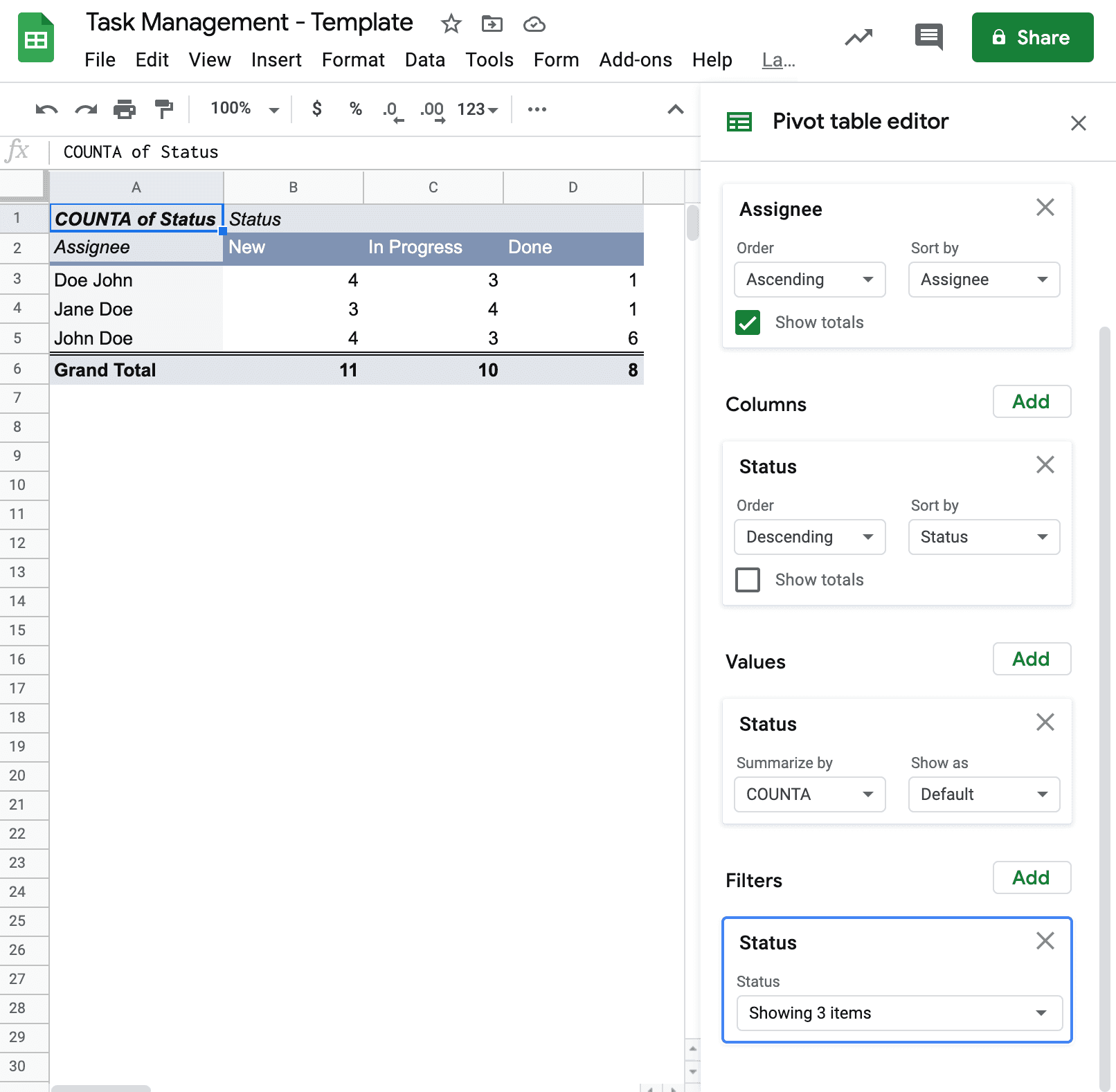
There you have it, a basic task management tool right in Google Sheets. There is a lot more that we can do with Google Sheets to make your task management tool robust and sophisticated.

In our next guide, we'll use it to manage all of our dropdowns in one place. Read our guide on advanced dropdowns