A Guide to Advanced Dropdowns in Google Sheets

In this short guide, we're going to learn how to use "Ranges" to make dynamic dropdowns in Google Sheets.

How will this make your spreadsheets better?

• It let's you control multiple dropdown values with ease
• It'll keep your sheet values nice and clean, which makes reporting easier
• You'll be able to scale the sheet with your team

Create a "Settings" tab

First step - let's create a new tab called "Settings". If you did this in A Guide to Task Management then you should already have it. If not, just click on the "+" icon in the footer to create a new tab and rename it to "Settings".

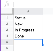
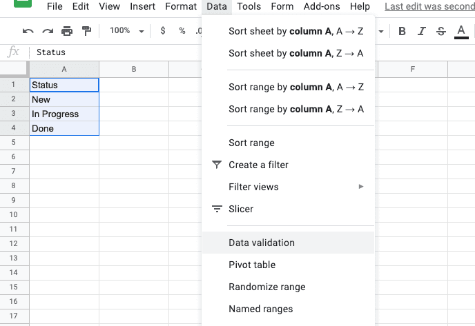
Once you're in your "Settings" tab, go to cell A1 (the first cell in the first column, in the first row). In our example, we'll just do a simple "Status" dropdown. Go ahead and type in "Status" for cell A1, "New" in cell A2, "In Progress" in cell A3, and "Done" in cell A4. It should look like this:

Create a Named Range

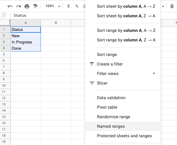
Highlight cells A1 through A4 and then select "Data" from the menu bar, and then select "Named ranges" from the list. This will open up a "tray" on the right hand side.

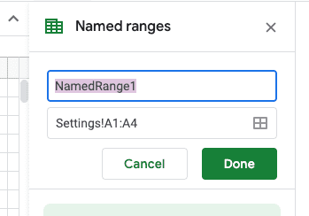
Since you highlighted A1:A4, the cell range field should be pre-populated for you. In the first field (it sould have defaulted to "NamedRange1"), just rename that to "Status".

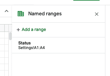
Once you've renamed it and saved the Named Range, the right-hand tray should update to show you the list of your Named Ranges. Since we just have one, you should only see "Status" in this list.

Update your Data Validation Dropdown

Now that you have a Named Range with your results, you can use it in your Data Validation options. Let's go back to your "Tasks" tab and highlight the column with your "Status". (if didn't complete our Guide to Task Management just highlight any column).

Once highlighted, click on the "Data" option in your menu bar and select "Data Validation.

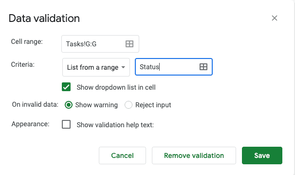
Since you highlighted your "Status" column, it should pre-populate into the "Cell range" field. In the "Criteria" field, select "List from a range" as the option and then type in "Status" in the field. This will have the Google Sheet read everything in the Named Range we just created.

Dynamic Ranges

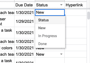
The beauty of using a Named Range is that you can update it without having to change your Data Validation settings. Give it a try by going back to your "Settings" tab and inserting a new row within your Named Range:

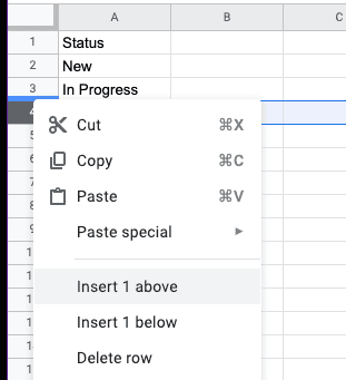
Let's call this new option "In Review"

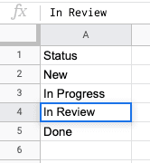
Since you inserted a new row within the Named Range, Google Sheets will automatically update everything for you. It should look like this for you now:

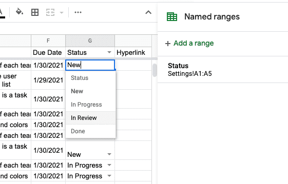
Now that you know how to set up Named Ranges in your Google Sheet, you'll be able to create sophisticated Google Sheet apps that you can manage at scale. Check out some of our other content to see what else you can do with Named Ranges.

In our next guide, we'll go back to our Task Management tool and start creating some alerts to help us stay on top of everything. Continue to our guide on Dynamic Alerts.